Map

For a while now, I've wanted to make some of the great functionality of things like Octave (and it's parent Matlab) to Common Lisp.  Mostly, I want things like the slice assignments (arrays with ranges in the indices) and matrix math.  Also, it never hurts to make higher mathematical functions available in simple ways.  So, I started writing Map, which I hope will do just that.

Lately, I've been working in singular optics, largely with Spatial Light Modulators, which are like very tiny LCD screens in front of a mirror. They're cool because they can transform the wavefront of a laser beam into any sort of beam you'd like!  We use a fair bit of math to pump out the right images to put onto the SLM, and I'd been wanting to make a more general interface for that for a while.  I'm not there yet, but I'd like to share the few things I've done so far.

Vectors

In Octave, you can type

[1:10]

and it will automatically be expanded to

[1 2 3 4 5 6 7 8 9 10]

.  This is great notation and can be used both for generating a vector or setting a range.  In map, I've implemented those with

#r(1 10)

, which creates a 'range' class that just keeps track of the numbers, and #v(1 10), which will expand to

#(1 2 3 4 5 6 7 8 9 10)

, like the Octave code.  This means you can do things like

(reduce #'+ #v(1 100))

To add up the numbers 1 to 100.  That, of course, isn't hard, especially when Gauss came up with a much easier way, but you get the picture.

One further thing that's special, is that you can apply a function to the vector you're generating by passing another argument (you can also pass a step size by entering three numbers).

(reduce #' #v(1 .1 10 #'sin))

will give you the sum of the sine of the numbers 1, 1.1, ..., 9.9, 10!  Moving on...

Differential Equations

This is a much more meaty section, and was really fun for me, since I hadn't really implemented a ODE solver before (that I remember).  Map now contains a Runge-Kutta Feldberg 45 solver, which is supposed to have an adaptive step size, and currently doesn't seem to, so I didn't do everything right, but it works to a certain accuracy.

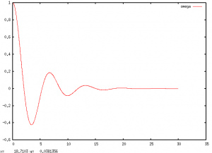
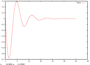
Here's a demonstration of finding the angular position and velocity ($\theta, \omega$) of a damped, driven pendulum, taken from some of my old computational physics notes.

(defun damped-pendulum (ti yi)
        (declare (type double-float ti)
                 (type (array double-float 2))
                 (ignore ti))
        (vector (+ (* -1d0 (sin (elt yi 1))) (* -1d0 .5d0 (elt yi 0)))
                (elt yi 0)))

(map::mute (multiple-value-setq (ts ys)
         (map:rkf45 #'damped-driven-pendulum
                #r(0d0 1d-7 4d1)
            #(0d0 1d0) 1d-10)))

Now, ts holds the time values, and ys is a 2x(length ts) array of position and velocity values!  Once I implement array slices, it'll be easy to graph them, but for now, you need to manually extract one of the rows of ys to plot against ts. There's still a lot of work to be done. Anyway, the resulting graphs are:

Thanks for reading, I'll probably post more once I've got slices sorted out.